🌡️ Surface Aerometry & Meteorological Instrumentation Monograph
An exhaustive engineering and physical treatise on in situ surface weather observations. We evaluate the architecture of Automated Surface Observing Systems (ASOS/AWOS), WMO exposure standards, precision platinum thermometry, resonant quartz barometry, acoustic ultrasonic anemometry, optical nephelometers, and laser ceilometers.
The global meteorological infrastructure rests upon the accuracy and temporal fidelity of in situ surface measurements. From international airport hubs where aircraft safety hinges upon exact runway visibility and wind shear reports, to agricultural regions monitoring frost conditions, surface observations provide the empirical bedrock of atmospheric science. In dynamic meteorology, surface observations represent the lower boundary condition for all atmospheric thermodynamic and fluid kinematic equations. Without continuous, standardized surface ground truth, global numerical weather models would diverge into chaos within hours.
Over the past four decades, surface meteorology has undergone a profound technological revolution: transitioning from manual, human-observed instruments to fully autonomous, solid-state measurement platforms known as the Automated Surface Observing System (ASOS) and Automated Weather Observing System (AWOS). Operating 24 hours a day, 365 days a year in extreme environments—from blistering desert heat exceeding 50°C to sub-zero polar blizzards below -50°C—these automated station networks measure, compute, encode, and transmit standardized meteorological reports (METAR and SPECI) to the global telecommunication grid every minute.
1. Standard Siting and Exposure Criteria: World Meteorological Organization (WMO) Guidelines
A meteorological sensor is only as accurate as its environmental exposure. If a precision thermometer is placed over asphalt or in the stagnant aerodynamic wake of a building, it will record microclimatic thermal artifacts rather than representative atmospheric state variables. Consequently, the World Meteorological Organization (WMO Technical Commission for Instruments and Methods of Observation, CIMO) and national aviation authorities enforce strict siting standards for official observation stations:
| Sensor / Parameter | Standard Operating Elevation | Required Distance from Obstacles | Underlying Ground Surface | Physical Rationale |
|---|---|---|---|---|
| Ambient Temperature & Humidity | 1.25 to 2.0 meters (4 to 6.5 ft) above ground | At least 4 times the height of the nearest obstacle | Natural, well-maintained short grass or natural native soil | Avoids extreme thermal microclimates within the laminar ground skin layer and artificial radiation |
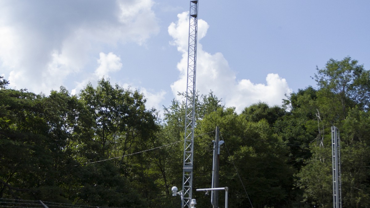
| Wind Speed and Direction | 10.0 meters (33 ft) above open terrain | At least 10 times the height of any obstruction within 300 meters | Open, unobstructed flat terrain | Eliminates aerodynamic surface boundary friction and obstacle-induced mechanical turbulence eddies |
| Precipitation Gauges | 0.5 to 1.5 meters above ground orifice | Protected from wind shear by Alter or Tretyakov wind shields | Natural sod or soil | Reduces aerodynamic wind undercatch; wind turbulence around gauge orifices can deflect up to 50% of falling snowflakes |
| Barometric Pressure Transducer | Station elevation calibrated to the nearest 0.1 meter | Enclosed within temperature-controlled, vented indoor shelter | Station indoor electronics rack | Protects against dynamic wind pressure fluctuations (pitot dynamic head effects via static pressure ports) |
2. Precision Temperature and Moisture Metrology
Modern automated stations have retired liquid-in-glass mercury thermometers in favor of solid-state Platinum Resistance Thermometers (PRTs), typically utilizing the standardized Pt100 or Pt1000 sensor configuration. The operating physical principle is based on the predictable, linear increase in the electrical resistance of pure platinum wire as thermal molecular vibrations impede electron flow, governed by the Callendar-Van Dusen equation:
R(T) = R_o * ( 1 + A * T + B * T^2 )
where R_o is the resistance at 0°C (precisely 100 ohms for a Pt100 element), and A and B are calibration coefficients. PRT sensors achieve extraordinary measurement precision (within ±0.05°C). To eliminate radiant solar heating artifacts, the PRT element is housed inside an aerodynamically ventilated radiation shield—either an aspiration chamber powered by a continuous electric fan or a stacked multi-plate louvred shield coated with ultra-high albedo titanium dioxide paint.
Atmospheric moisture is measured using thin-film capacitive polymer hygrometers. A microscopic hygroscopic dielectric polymer layer is sandwiched between two porous gold electrode films. As environmental water vapor molecules diffuse through the gold electrode, the polymer absorbs moisture in direct thermodynamic equilibrium with the ambient relative humidity, altering the electrical capacitance of the sensor chip. For high-precision climate reference stations, capacitive sensors are supplemented by chilled-mirror optical dewpoint hygrometers, which actively chill a rhodium-plated copper mirror via a thermoelectric Peltier cooler until microscopic dew or frost condensation forms, detecting the exact phase change optically via phototransistors to determine the dewpoint temperature within ±0.1°C.
3. Precision Barometry and Altimetry Reduction Mathematics
Barometric pressure is the single most critical thermodynamic variable measured at the surface. Modern ASOS stations employ triply redundant Resonant Quartz Crystal Pressure Transducers. Atmospheric pressure is ported to a precision silicon diaphragm coupled to an oscillating quartz crystal beam. As barometric pressure varies, the mechanical stress applied to the quartz crystal changes its resonant piezoelectric oscillation frequency. By measuring this resonant frequency with high-precision quartz clock counters, pressure is resolved to an astonishing 0.01 hectopascal (hPa) with virtually zero long-term sensor drift.
Because stations are located at varying elevations above sea level, raw station pressure (P_station) must be mathematically reduced to standardized reference datums using the Hypsometric Equation:
P_0 = P_station * exp( (g * h_station) / (R_d * bar(T_v)) )
Operational aviation and synoptic meteorology utilize three distinct pressure reductions:
- Altimeter Setting (QNH): The barometric pressure reduced to sea level using the standard ICAO standard atmosphere (assuming a constant lapse rate of 6.5°C/km and standard sea-level temperature of 15°C). Altimeter settings are used by aircraft barometric altimeters to ensure vertical terrain clearance and air-traffic separation.
- Sea-Level Pressure (SLP / QFF): The pressure reduced to sea level utilizing the true, 12-hour averaged environmental surface virtual temperature (bar(T_v)) to account for real-world boundary-layer air density. SLP is the universal variable plotted on synoptic surface weather maps to analyze isobars, cyclones, and anticyclones.
- QFE: Unreduced station pressure, indicating the actual barometric weight of the air resting on the runway threshold, causing an aircraft altimeter to read exactly zero upon touchdown.
4. Anemometry: Mechanical vs. Three-Dimensional Sonic Anemometers
For over a century, surface wind measurements relied on mechanical Robinson cup anemometers for wind speed and counterbalanced wind vanes for direction. However, mechanical sensors suffer from unavoidable physical inertia:
- They possess a mechanical starting threshold (typically 0.5 to 1.0 m/s) below which light winds cannot overcome bearing friction.
- During turbulent wind gusts, mechanical cups accelerate faster than they decelerate (an aerodynamic bias termed ‘cup overspeeding’), systematically overestimating mean turbulent wind speeds.
- Mechanical bearings and cup assemblies are highly vulnerable to freezing rain and riming ice accretion, which immobilizes moving parts during severe winter storms.
Modern ASOS networks have transitioned to solid-state Ultrasonic Sonic Anemometers. A sonic anemometer measures wind velocity by emitting high-frequency acoustic ultrasound pulses (typically 100 kHz) across paired piezoelectric transducers separated by a fixed distance d (typically 10 to 20 cm). The transit time of sound traveling with the wind (t_1) is shorter than the transit time traveling against the wind (t_2):
t_1 = d / (c_s + v) quad text{and} quad t_2 = d / (c_s – v)
Solving simultaneously for the wind component v along the transducer axis yields:
v = (d / 2) * [ (1 / t_1) – (1 / t_2) ]
Notice that this equation is completely independent of the speed of sound c_s in air (and therefore independent of air temperature, humidity, and density). By arranging three orthogonal pairs of ultrasonic transducers, the instrument measures the complete three-dimensional wind vector (u, v, w) at sampling frequencies up to 50 Hz with zero moving parts, instantaneous response, and internal electrical heating elements that melt freezing rain without interrupting operational telemetry.
5. Optical Hydrometeor and Cloud Base Detection: Nephelometers and Ceilometers
Automating visibility and cloud height determinations required breakthrough innovations in optical physics:
| Automated Optical Sensor | Operating Physical Principle | Target Meteorological Variable | Aviation & Weather Utility |
|---|---|---|---|
| Forward-Scatter Present Weather Sensor (Nephelometer) | Infrared LED beam (lambda = 880 nm) scattered forward at 33° angle into a photodiode detector | Meteorological Optical Range (Visibility from 10 m to 50 km) and precipitation identification | Measures extinction coefficient; distinguishes rain, drizzle, and snow based on optical pulse amplitude signatures |
| Laser Ceilometer (LIDAR) | Pulsed semiconductor diode laser (lambda = 905 nm) firing vertically; measures time-of-flight of backscattered photon pulses | Cloud base height (ceiling) and vertical cloud layer stratification up to 25,000 feet (7,500 m) | Time-resolved backscatter profiles detect multiple cloud layers, aerosol layers, and vertical visibility in dense fog |
| Freezing Rain Sensor | Ultrasonically vibrating magnetostrictive resonant oscillator probe (40 kHz) | Accretion of supercooled freezing rain / drizzle ice | Ice freezing onto the probe increases its mass, dampening the resonant vibration frequency to trigger automated cockpit icing alerts |
| Automated Lightning Sensor | Combined magnetic direction finder (VLF/LF) and electrostatic field mill | Thunderstorm onset, cloud-to-ground lightning range and bearing within 30 nautical miles | Automates TS (Thunderstorm) code insertion into METAR aviation observation streams |
6. Precipitation Measurement: Tipping-Bucket vs. Precision Weighing Gauges
Liquid and solid precipitation accumulation is measured through two primary sensor paradigms:
- Tipping-Bucket Rain Gauges: Precipitation falling into an 8-inch calibrated collector funnel is directed onto a balanced two-compartment seesaw bucket. When precisely 0.01 inches (0.25 mm) of water fills the active compartment, gravity tips the bucket, emptying the water and momentarily closing a magnetic reed switch that records a digital electrical pulse. While mechanically simple, tipping-bucket gauges systematically undercount intense tropical downpours due to water loss during the physical tipping motion, and are completely incapable of measuring snowfall without electric heating grids that cause evaporative losses.
- All-Weather Weighing Precipitation Gauges: Modern stations employ high-precision electronic load-cell weighing gauges (such as the OTT Pluvio). Falling precipitation—whether liquid rain, freezing drizzle, graupel, or heavy snow—drops directly into an antifreeze and oil-shielded bucket suspended on temperature-compensated strain-gauge load cells. The instrument measures the total mass increase continuously at a resolution of 0.001 mm. By measuring mass directly rather than volume, weighing gauges eliminate tipping losses, measure dry snowfall with millimeter precision, and provide instantaneous precipitation intensity rates with unmatched scientific accuracy.
7. Micrometeorological Flux Towers and Eddy Covariance
Beyond standard operational ASOS networks, advanced atmospheric research relies on Micrometeorological Flux Towers operating via the Eddy Covariance Method. These specialized installations measure the turbulent vertical exchange of sensible heat, latent heat (evapotranspiration), momentum, and trace greenhouse gases (CO2, CH4, and H2O) between the terrestrial biosphere and the lower atmosphere.
By pairing high-frequency three-dimensional sonic anemometers (sampling at 10 to 20 Hz) with open-path or closed-path infrared gas analyzers (IRGAs), the instrument suite computes instantaneous Reynolds stress terms and covariance products:
H = rho * c_p * bar(w’ T’) quad text{and} quad LE = rho * L_v * bar(w’ q’)
where bar(w’ T’) is the turbulent vertical heat flux and bar(w’ q’) is the moisture flux. Eddy covariance towers (such as those maintained globally by FLUXNET and the National Ecological Observatory Network, NEON) provide ground-truth boundary-layer flux validations that parameterize land-surface interaction models within global numerical climate models.
8. The Future of Ground Observations: Dense Mesonets and Crowdsourced Telemetry
As numerical weather models advance toward convection-allowing grid resolutions of 1 kilometer or less, the traditional spacing of airport ASOS stations (typically 50 to 100 kilometers apart) is insufficient to resolve fine-scale thunderstorm cold pools, agricultural microclimates, and complex terrain winds. To solve this spatial undersampling, meteorologists are deploying dense statewide Mesonets—such as the celebrated Oklahoma Mesonet and New York State Mesonet—which maintain automated stations every 20 to 30 kilometers across entire states.
Simultaneously, the integration of crowdsourced pressure telemetry from barometric sensors embedded in millions of consumer smartphones and connected vehicles represents a transformative observational frontier. Machine learning quality-control algorithms filter out artificial indoor and motion artifacts, yielding massive, high-density surface pressure networks that detect propagating thunderstorm gust fronts and gravity waves with unprecedented spatial fidelity, bridging the gap between classical meteorological instrumentation and modern big-data atmospheric science.
9. Sub-Surface Agro-Meteorological Arrays: Soil Temperature & Moisture Dynamics
Complete surface meteorological characterization requires examining the thermodynamic properties of the underlying soil substrate. Automated networks (such as the Soil Climate Analysis Network, SCAN, and agricultural mesonet extensions) deploy subterranean multi-depth sensor arrays typically buried at 5 cm, 10 cm, 20 cm, 50 cm, and 100 cm depths.
Soil moisture is determined using Time-Domain Reflectometry (TDR) or coaxial impedance probes. The instrument transmits an ultra-fast electrical pulse along parallel stainless steel waveguide rods inserted into the soil. Because the dielectric permittivity of liquid water (~ 80) is dramatically higher than that of dry soil mineral matrix (~ 3 to 5) and air (~ 1), the propagation velocity of the electromagnetic pulse is dictated almost exclusively by the volumetric water content (VWC, expressed in m³/m³). Concurrently, precision thermistors embedded at each depth profile the vertical diffusion of the diurnal solar thermal wave through the ground, measuring soil thermal conductivity and heat flux parameters vital for frost depth prediction, agricultural planting windows, and hydrological land-atmosphere coupling.